Imagine adjusting the focus of a camera lens: a wide aperture captures more details but risks blurring the image, while a narrow aperture misses finer details but ensures sharpness. Similarly, Vapnik-Chervonenkis (VC) capacity is like a lens for machine learning models, determining their ability to capture patterns and generalize without overfitting or underfitting.

A Brief History of VC Capacity
Developed in 1971 by Vladimir Vapnik and Alexey Chervonenkis, VC capacity emerged as a pivotal concept in statistical learning theory. It laid the groundwork for Support Vector Machines (SVMs) and other modern machine learning algorithms. Today, VC capacity is critical in designing models that strike the right balance between complexity and generalization.
What Is Vapnik-Chervonenkis Capacity?
VC capacity measures the complexity of a model’s hypothesis space—the set of functions it can learn. It evaluates how many data points a model can “shatter,” or perfectly classify, no matter how they are arranged.
For example:
- A straight line has a low VC capacity, as it can only separate linearly separable data.
- A complex neural network has a high VC capacity, capable of classifying intricate patterns.
Think of VC capacity as the aperture of a camera lens: too wide, and the image (model) overfits by capturing every detail, including noise; too narrow, and it underfits by missing critical details.
Why Is VC Capacity Used?
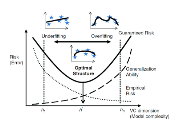
VC capacity is essential for balancing underfitting and overfitting in machine learning:
- Underfitting: Models with low VC capacity fail to capture the complexity of the data.
- Overfitting: Models with high VC capacity memorize the training data, reducing their ability to generalize.
- Generalization: VC capacity ensures models perform well on new, unseen data.
For instance, in fraud detection, models with the right VC capacity can identify fraudulent patterns without flagging legitimate transactions as suspicious.
How Is VC Capacity Used?
Machine learning practitioners use VC capacity in several ways:
- Model Selection: Choosing models with appropriate complexity for the dataset.
- Hyperparameter Tuning: Adjusting parameters like tree depth or neural network layers to optimize capacity.
- Validation Techniques: Using methods like cross-validation to evaluate model generalization.
VC capacity is particularly important in algorithms like SVMs, decision trees, and deep learning models.
Types of VC Measures
- Empirical VC Dimension: Derived from specific data and hypothesis class.
- Theoretical VC Dimension: A broader measure independent of specific datasets.
Categories of Models Based on VC Capacity
- Low VC Capacity Models: Linear regressions and shallow decision trees (prone to underfitting).
- High VC Capacity Models: Complex neural networks and polynomial regressions (risk of overfitting).
Software and Tools for VC Analysis
Although VC capacity isn’t directly computed in standard tools, related functionalities are available in:
- Scikit-learn: Tools for cross-validation and regularization to manage capacity.
- TensorFlow/Keras: Frameworks for designing models with controlled capacity.
- R Programming: Libraries for model evaluation and generalization testing.
Industry Applications in Australian Governmental Agencies
- Healthcare Analytics: The Australian Institute of Health and Welfare employs VC-informed models to predict disease trends, ensuring balanced accuracy and reliability.
- Environmental Resource Management: Geoscience Australia uses VC-based models to analyze satellite imagery for resource allocation, improving decision-making across diverse regions.
- Traffic Optimization: Transport for NSW applies machine learning models with optimal VC capacity to predict traffic flow patterns, enabling efficient public transport management.
How interested are you in uncovering even more about this topic? Our next article dives deeper into [insert next topic], unravelling insights you won’t want to miss. Stay curious and take the next step with us!