A Very Short Introduction of Markov Random Fields (MRF)

A Brief History of This Tool: Who Developed It?

Markov Random Fields (MRFs) were developed as a probabilistic graphical model rooted in the work of Andrey Markov in the early 20th century. Later advancements by researchers like Julian Besag in the 1970s and 1980s formalised MRFs for modern computational applications, especially in the fields of image processing and spatial statistics.

 

What Is It?

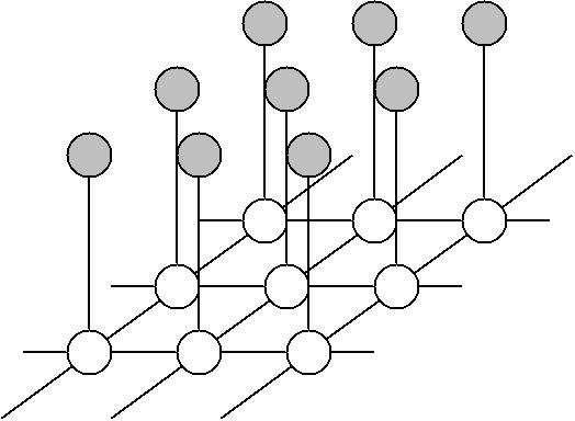
Imagine a sprawling neighbourhood where the state of one house (like its cleanliness) depends not only on its occupants but also on the state of its neighbouring houses. Similarly, MRFs model the relationships between variables, capturing dependencies within a network of nodes, where each node interacts with its neighbours.

An MRF is a probabilistic graphical model that represents the joint distribution of a set of random variables through a graph structure. The edges of the graph define the conditional dependencies between the variables.

Why Is It Being Used? What Challenges Are Being Addressed?

MRFs shine in areas where spatial or contextual relationships are critical. Key applications include:

• Image Denoising and Segmentation: Enhancing image clarity by modelling pixel dependencies.
• Natural Language Processing: Understanding syntactic and semantic structures.
• Data Labelling: Ensuring contextual consistency in structured prediction tasks.

Global Impact: MRFs are widely employed in AI applications globally. Research from Markets and Markets predicts that the AI-driven image recognition market, a prime user of MRFs, will grow to $76 billion by 2030.

Australia: MRFs are used by agencies like CSIRO for environmental modelling and satellite image analysis, contributing to 20% faster land-use classification.

How Is It Being Used?

MRFs are utilised by:

1. Building Probabilistic Models: Representing variables in a system and their dependencies.
2. Inference: Using algorithms like Gibbs Sampling to determine the probable states of the variables.
3. Learning Parameters: Estimating graph weights from data for better prediction accuracy.

Different Types

MRFs have several key variations:

• Ising Model: A specific type of MRF used for binary variables, often in physics.
• Gaussian MRF: Used for continuous random variables, ideal for spatial data.
• Conditional Random Fields (CRFs): A related model focusing on discriminative learning.

Different Features

Key features of MRFs include:

• Graphical Representation: Nodes and edges form an intuitive framework for modelling dependencies.
• Flexibility: Applicable across discrete and continuous data.
• Local Markov Property: Simplifies computations by leveraging conditional independence.

Different Software and Tools for MRFs

Developers can use the following tools to implement MRFs:

• PyMC3: Bayesian modelling library supporting MRFs.
• Stan: Probabilistic programming language for graphical models.
• OpenCV: Contains implementations for MRF-based image processing tasks.

Industry Application Examples in Australian Governmental Agencies

1. CSIRO:
   • Use Case: Land-use mapping from satellite imagery.
   • Impact: Achieved 20% faster classification and improved conservation planning.
2. Australian Bureau of Statistics (ABS):
   • Use Case: Spatial data modelling for population density predictions.
   • Impact: Enhanced accuracy in urban planning reports.
3. Geoscience Australia:
   • Use Case: Modelling geological structures and resource distribution.
   • Impact: Accelerated resource exploration by 15%.